
TensorFlow is an open-source software library for numerical computation, specifically designed for building and training machine learning models. It was developed by the Google Brain team and is now maintained by the TensorFlow development community. TensorFlow is widely used in industry and academia for a variety of machine learning tasks, including regression modeling.
A regression model is a type of machine learning model that is used to predict a continuous target variable based on one or more input features. In regression modeling, the goal is to learn a function that maps the input features to the target variable, using a set of training examples. The learned function can then be used to make predictions on new data.
TensorFlow provides a powerful and flexible framework for building and training regression models. It offers a wide range of tools for constructing and manipulating mathematical expressions, including automatic differentiation, which makes it easy to compute gradients for optimization. TensorFlow also provides a variety of pre-built layers and functions for building different types of neural networks, including feedforward networks, convolutional networks, and recurrent networks, which can be used for regression modeling.
To build a regression model using TensorFlow, one typically defines a neural network architecture that maps the input features to the target variable, and then trains the model using a training dataset. During training, the model adjusts its parameters to minimize a loss function that measures the difference between the predicted and actual target values. Once trained, the model can be used to make predictions on new data.
Building a Regression model using TensorFlow
Here’s an example code for building a regression model using TensorFlow, along with an existing dataset. In this example, we use the “Appliances energy prediction” dataset from the UCI Machine Learning Repository (https://archive.ics.uci.edu/ml/datasets/Appliances+energy+prediction). The dataset contains 19735 samples with 29 features and a target variable (Appliances energy consumption in Wh).
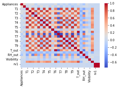
We can use heatmaps to visualize the “Appliances energy prediction” dataset. Heatmaps are useful when we want to visualize the correlation between different features of the dataset.
import pandas as pd
import seaborn as sns
import matplotlib.pyplot as plt

# Load the dataset
df = pd.read_csv("https://archive.ics.uci.edu/ml/machine-learning-databases/00374/energydata_complete.csv")

# Drop the date column, as they are not relevant for the visualization
df = df.drop(columns=["date"])

# Compute the correlation matrix
corr = df.corr()

# Create a heatmap of the correlation matrix
sns.heatmap(corr, cmap="coolwarm", )

# Show the plot
plt.show()
The resulting heatmap will show the correlation between each pair of features in the dataset, with positive correlations in red and negative correlations in blue. Features that are highly correlated will be close to each other on the heatmap.
We load the dataset using Pandas and split it into training and testing sets using Scikit-learn‘s train_test_split function. We then normalize the data using Scikit-learn’s MinMaxScaler.
import tensorflow as tf
import numpy as np

# Load the dataset
data = pd.read_csv('https://archive.ics.uci.edu/ml/machine-learning-databases/00374/energydata_complete.csv')
x = data.drop(['date', 'Appliances'], axis=1).values
y = data['Appliances'].values

# Split the data into training and testing sets
from sklearn.model_selection import train_test_split
x_train, x_test, y_train, y_test = train_test_split(x, y, test_size=0.2, random_state=42)

# Normalize the data
from sklearn.preprocessing import MinMaxScaler
scaler = MinMaxScaler()
x_train = scaler.fit_transform(x_train)
x_test = scaler.transform(x_test)
We build a simple neural network model with two hidden layers of 64 neurons each, with ReLU activation functions. The output layer has a single neuron for the regression task. We compile the model with the mean squared error loss function and the adam optimizer. We then train the model for 100 epochs with a batch size of 64.
# Build the model
model = tf.keras.models.Sequential([
    tf.keras.layers.Dense(units=64, activation='relu', input_shape=(x_train.shape[1],)),
    tf.keras.layers.Dense(units=64, activation='relu'),
    tf.keras.layers.Dense(units=1)
])

model.compile(optimizer='adam', loss='mse', metrics='mse')

# Train the model
history = model.fit(x_train, y_train, epochs=100, batch_size=64, validation_data=(x_test, y_test))
Finally, we evaluate the model on the testing set using the mean squared error metric. The trained model can be used to make predictions on new data.
# Evaluate the model
loss, mse = model.evaluate(x_test, y_test)
print('Test MSE: {:.2f}'.format(mse))
Here’s an example code to plot the loss and mean squared error (MSE) during training of a regression model built using TensorFlow:
import matplotlib.pyplot as plt

# Plot the loss and MSE curves
plt.figure(figsize=(10, 5))
plt.plot(history.history['loss'], label='Training Loss')
plt.plot(history.history['val_loss'], label='Validation Loss')
plt.plot(history.history['mse'], label='Training MSE')
plt.plot(history.history['val_mse'], label='Validation MSE')
plt.title('Training and Validation Loss and MSE')
plt.xlabel('Epoch')
plt.ylabel('Loss/MSE')
plt.legend()
plt.show()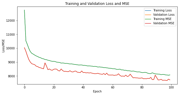
MSE stands for Mean Squared Error, and it is a common metric used to evaluate the performance of regression models. It measures the average squared difference between the predicted values and the actual values. In other words, it calculates the average of the squared residuals, which is the difference between the predicted and actual values for each data point in the dataset.
The formula for calculating MSE is:
MSE = (1/n) * Σ(yᵢ – ȳ)²
where:
- n is the number of data points
- yᵢ is the predicted value for the i-th data point
- ȳ is the actual (or target) value for the i-th data point
MSE is a non-negative value, where a lower value indicates better performance. It is commonly used as the loss function for regression models, which means that during training, the model tries to minimize the MSE by adjusting its parameters to improve the predictions.
Tips for Regression modeling
Here are some tips for building effective regression models:
- Understand your data: Before building a regression model, it’s important to have a good understanding of the data you’re working with. This includes exploring the data to understand the relationships between the input features and the target variable, as well as identifying any missing values, outliers, or other data quality issues that may impact the performance of the model.
- Choose appropriate features: The choice of input features is a critical factor in building an effective regression model. It’s important to select features that are relevant to the problem you’re trying to solve and that capture the underlying patterns and relationships in the data. It can be helpful to use domain knowledge or feature engineering techniques to create new features that may be more informative for the target variable.
- Normalize the data: Normalizing the input features can help improve the performance of regression models. This can be done by scaling the features so that they have a mean of zero and a standard deviation of one, or by using other normalization techniques such as min-max scaling or z-score scaling.
- Choose an appropriate loss function: The choice of loss function can have a significant impact on the performance of the model. For regression tasks, common loss functions include mean squared error (MSE) and mean absolute error (MAE). MSE tends to be more sensitive to outliers, while MAE is more robust to outliers.
- Choose an appropriate optimization algorithm: The choice of optimization algorithm can also impact the performance of the model. Common optimization algorithms for regression modeling include stochastic gradient descent (SGD) and its variants, such as Adam and Adagrad. It can be helpful to experiment with different optimization algorithms and learning rates to find the one that works best for your particular problem.
- Regularize the model: Regularization techniques, such as L1 and L2 regularization, can help prevent overfitting and improve the generalization performance of the model. It’s important to choose an appropriate regularization strength that balances the bias-variance tradeoff.
- Evaluate the model: Evaluating the performance of the model on a validation set or through cross-validation is critical for understanding how well the model is likely to perform on new data. It’s important to choose appropriate evaluation metrics that are relevant to the problem you’re trying to solve.
- Tune hyperparameters: Finally, it’s important to experiment with different hyperparameters, such as the number of layers and neurons in the network, the batch size, and the regularization strength, to find the best set of hyperparameters for your particular problem. This can be done through a process of trial and error or by using automated hyperparameter tuning techniques.
Further readings
Here are some resources for further reading on TensorFlow and regression modeling:
- TensorFlow documentation – https://www.tensorflow.org/api_docs/python/ The official documentation for TensorFlow provides a wealth of information about the library, including tutorials and code examples for building regression models using TensorFlow.
- TensorFlow for Deep Learning: From Linear Regression to Reinforcement Learning – https://www.amazon.com/TensorFlow-Deep-Learning-Regression-Reinforcement/dp/1491980451/ This book by Bharath Ramsundar and Reza Bosagh Zadeh provides a comprehensive guide to using TensorFlow for deep learning, including regression modeling. It covers a wide range of topics, from linear regression to reinforcement learning, and includes numerous code examples and case studies.
- Hands-On Machine Learning with Scikit-Learn, Keras, and TensorFlow – https://www.amazon.com/Hands-Machine-Learning-Scikit-Learn-TensorFlow/dp/1492032646/ This book by Aurélien Géron provides a practical guide to machine learning using scikit-learn, Keras, and TensorFlow. It includes a section on regression modeling with TensorFlow, as well as coverage of many other topics, including classification, clustering, and deep learning.
- Regression with TensorFlow – https://www.tensorflow.org/tutorials/keras/regression This tutorial on the official TensorFlow website provides a step-by-step guide to building a regression model using TensorFlow and Keras. It includes code examples and explanations of the key concepts involved in building a regression model, including normalization, loss functions, and optimization algorithms.
- Regression Modeling with TensorFlow – https://www.youtube.com/watch?v=MrLPzBxQ6yE This video by Packt Publishing provides an overview of how to build a regression model using TensorFlow, including data preprocessing, model construction, and training. It also covers topics such as overfitting and model evaluation.
These resources should provide a good starting point for learning more about TensorFlow and regression modeling. Good luck!