A Simple Guide to Convolutional Neural Networks

Convolutional Neural Networks (CNNs) have revolutionized the field of deep learning in recent years. They are a type of neural network that is especially effective for image recognition tasks, but can also be applied to other types of data, such as audio and text. In this article, we will provide a simple guide to CNNs, including an overview of the architecture, the training process, and some practical applications. We will also include some code examples in Python using the popular deep learning library, TensorFlow.

Overview of Convolutional Neural Networks

At a high level, a CNN consists of several layers that are designed to process and transform input data. The key layers of a typical CNN are:

1. Convolutional layer – applies a set of filters to the input image to extract features.
2. Pooling layer – reduces the size of the feature maps by downsampling them.
3. Fully connected layer – connects the output of the previous layers to a set of output nodes that produce the final classification result.

The architecture of a CNN can be visualized as a series of 2D matrices (also known as tensors) that flow through the different layers, with each layer performing a specific type of transformation. The input tensor is typically a 3D matrix with dimensions (height, width, channels), where channels refer to the number of color channels in the image (e.g., 3 for RGB images).

You can view 2D visualization of the CNN network in this site.

Training a Convolutional Neural Network

The training process for a CNN is similar to that of other neural networks, in that it involves backpropagation and gradient descent to optimize the network’s parameters. However, there are a few key differences in how CNNs are trained compared to other neural networks:

1. The use of convolutional and pooling layers allows the network to learn spatially invariant features, meaning that it can recognize the same object regardless of where it appears in the image.
2. Data augmentation techniques such as random cropping, flipping, and rotation can be used to artificially increase the size of the training dataset and improve the network’s ability to generalize to new images.
3. Transfer learning, which involves reusing pre-trained networks and fine-tuning them on a new dataset, is often used to speed up the training process and improve the network’s performance.

Practical Applications of Convolutional Neural Networks

CNNs have numerous practical applications, some of which include:

1. Image classification – recognizing objects in images
2. Object detection – locating and identifying objects in images
3. Semantic segmentation – segmenting images into regions that correspond to different objects or parts of objects
4. Image generation – generating new images that resemble a given dataset
5. Style transfer – applying the style of one image to another image

Code Examples in Python

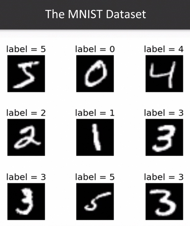
To demonstrate the implementation of a CNN in Python using TensorFlow, we will use the MNIST dataset, which consists of 28×28 grayscale images of handwritten digits.

First, we will import the necessary libraries and load the dataset:

import tensorflow as tf
from tensorflow.keras.datasets import mnist

(x_train, y_train), (x_test, y_test) = mnist.load_data()

Next, we will preprocess the data by normalizing the pixel values and adding an extra dimension to the input tensors to make them compatible with the Conv2D layer in the CNN. The ‘...' syntax is used to indicate that all the existing dimensions of the tensor should be preserved, and a new dimension should be added at the end. The tf.newaxis function is a shorthand for tf.newaxis, which creates a new axis of size 1 at the specified position in the tensor. In this case, we are adding a new axis at the end of the tensors.

x_train = x_train.astype('float32') / 255.0
x_test = x_test.astype('float32') / 255.0

x_train = x_train[..., tf.newaxis]
x_test = x_test[..., tf.newaxis]

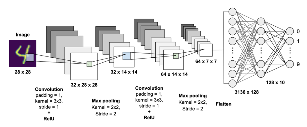
Then, we will define the CNN architecture using the Keras API, which is built into TensorFlow:

model = tf.keras.models.Sequential([
  tf.keras.layers.Conv2D(32, (3,3), activation='relu', input_shape=(28,28,1)),
  tf.keras.layers.MaxPooling2D((2,2)),
  tf.keras.layers.Conv2D(64, (3,3), activation='relu'),
  tf.keras.layers.MaxPooling2D((2,2)),
  tf.keras.layers.Flatten(),
  tf.keras.layers.Dense(128, activation='relu'),
  tf.keras.layers.Dense(10, activation='softmax')
])

This model consists of two sets of convolutional and pooling layers, followed by two fully connected layers. A Conv2D layer is a type of layer used in CNNs for image recognition and processing tasks. Conv2D stands for 2-dimensional convolution, which refers to the mathematical operation of sliding a small filter or kernel over the input image in order to extract features from it. The Conv2D layer applies this operation to the input image to produce a set of output feature maps.

The Conv2D layer takes as input a 3-dimensional tensor representing the image data (height, width, and number of channels), and applies a set of learnable filters to the input in order to extract important features. The filters, which are typically small squares of pixels, slide across the input image and perform a dot product with the corresponding pixels in the input image to produce a single value in the output feature map.

By stacking multiple Conv2D layers on top of one another, a CNN is able to extract increasingly complex and abstract features from the input image. These features can then be passed to a fully connected layer for classification or other downstream tasks.

MaxPooling2D is a layer used in CNNs for down-sampling or reducing the spatial dimensions of the feature maps produced by a Conv2D layer. The MaxPooling2D layer applies a max pooling operation to each feature map, where it divides the feature map into a set of non-overlapping rectangular regions or pooling windows, and outputs the maximum value within each window. This process effectively reduces the spatial size of the feature maps while preserving the most important features, and it helps to reduce the number of parameters in the model and prevent overfitting.

MaxPooling2D typically uses a square pooling window with a fixed size and stride. The pooling window size and stride are hyperparameters that can be specified by the user, and they determine the amount of down-sampling that occurs. A larger pooling window or stride size results in more aggressive down-sampling, while a smaller size results in more conservative down-sampling.

MaxPooling2D can be applied after one or more Conv2D layers in a CNN, and it is often used in conjunction with other types of layers such as activation layers, dropout layers, and fully connected layers to build more complex models.

The final output layer has 10 nodes, one for each possible digit class (0-9), and uses a softmax activation function to produce a probability distribution over the classes.

Next, we will compile the model, specifying the loss function, optimizer, and evaluation metric:

model.compile(optimizer='adam',
              loss='sparse_categorical_crossentropy',
              metrics=['accuracy'])

Sparse categorical cross-entropy is a loss function that is commonly used in machine learning for multi-class classification problems, where the number of classes is greater than two. The goal of the loss function is to measure the difference between the predicted probability distribution of the model and the actual probability distribution of the target classes.

The “sparse” part of the name comes from the fact that this loss function is used when the target variable is represented as a single integer, rather than a one-hot encoded vector. In other words, if the target class labels are represented as integers (e.g., 0, 1, 2, 3, etc.), rather than one-hot encoded vectors (e.g., [1, 0, 0], [0, 1, 0], [0, 0, 1], etc.), then the sparse categorical cross-entropy loss function can be used.

The sparse categorical cross-entropy loss function calculates the cross-entropy loss between the predicted probability distribution and the true probability distribution of the target classes. The true probability distribution is represented as a one-hot encoded vector, with a value of 1 for the true class and a value of 0 for all other classes. The predicted probability distribution is calculated by passing the input data through the model and using a softmax activation function to convert the final layer outputs into a probability distribution.

The final loss value is the average of the cross-entropy loss across all samples in the batch. The goal of training the model is to minimize this loss function, which encourages the model to make better predictions and improve its overall performance.

Finally, we can train the model on the MNIST dataset using the fit method:

model.fit(x_train, y_train, epochs=5, validation_data=(x_test, y_test))

After training for 5 epochs, we can evaluate the model’s performance on the test set using the evaluate method:

test_loss, test_acc = model.evaluate(x_test, y_test)
print('Test accuracy:', test_acc)

With just a few lines of code, we have trained a CNN that can classify handwritten digits with over 99% accuracy on the test set!

Conclusion

Convolutional neural networks are a powerful tool for image recognition and other types of data processing tasks. In this article, we provided a simple guide to CNNs, covering the architecture, training process, and practical applications. We also included some code examples in Python using TensorFlow to demonstrate how to implement a CNN for image classification. With the availability of powerful deep learning libraries such as TensorFlow, it is now easier than ever to get started with CNNs and explore their many applications.

Further readings

If you’re interested in learning more about convolutional neural networks and deep learning, here are some recommended resources:

1. “Deep Learning” by Ian Goodfellow, Yoshua Bengio, and Aaron Courville – this is a comprehensive textbook on deep learning that covers a wide range of topics, including CNNs.
2. “Convolutional Neural Networks for Visual Recognition” by Fei-Fei Li, Justin Johnson, and Serena Yeung – this is a popular course on CNNs from Stanford University, which includes lecture videos, slides, and assignments.
3. TensorFlow website – TensorFlow is a popular open-source deep learning library, which provides a wide range of resources and tutorials on CNNs and other deep learning topics.
4. PyTorch website – PyTorch is another popular open-source deep learning library, which has a user-friendly interface and is particularly well-suited for research applications.
5. Kaggle – Kaggle is a platform for data science competitions, where you can find a wide range of datasets and challenges related to CNNs and other deep learning topics. You can also access code examples and tutorials from other users.
6. ArXiv – ArXiv is a repository of preprints for scientific papers in a wide range of fields, including deep learning. You can search for papers related to CNNs and other deep learning topics and stay up-to-date with the latest research.