Simple Deep Learning Classification Model using TensorFlow

Deep learning is a subfield of machine learning that involves building and training neural networks, which are a type of computational model inspired by the structure and function of the human brain. In deep learning, neural networks are typically organized into multiple layers, with each layer consisting of a set of interconnected neurons that process and transform input data. By stacking multiple layers, deep neural networks can learn increasingly complex representations of the input data, enabling them to make highly accurate predictions and classifications.

TensorFlow is an open-source software library developed by Google that is widely used in deep learning applications. It provides a flexible and powerful framework for building and training neural networks, with support for a wide range of tasks, including classification, regression, and image and language processing. TensorFlow also provides a range of tools for optimizing and deploying deep learning models in production environments.

Classification is a fundamental problem in machine learning and deep learning, where the goal is to assign input data to one of several predefined categories or classes. In a classification problem, the input data is typically represented by a set of features or attributes, and the output is a categorical label that indicates which class the data belongs to. Neural networks are a popular approach for solving classification problems, as they can learn highly nonlinear and complex decision boundaries that can separate different classes of data.

In TensorFlow, you can build and train classification models using a wide range of neural network architectures, including fully connected networks, convolutional networks, and recurrent networks, among others. TensorFlow also provides a wide range of loss functions, optimization algorithms, and evaluation metrics that can be used to train and evaluate classification models, as well as tools for visualizing and analyzing the behavior of trained models. With its ease of use and flexibility, TensorFlow is an excellent choice for building and deploying deep learning models for a wide range of classification tasks.

Multilayer Perceptron

MLP stands for Multilayer Perceptron, which is a type of artificial neural network (ANN) that consists of multiple layers of interconnected perceptrons. A perceptron is a simple mathematical function that takes a set of inputs, applies weights to them, and outputs a single binary value. The weights are learned during the training process, which involves adjusting them to minimize the error between the predicted output and the actual output.

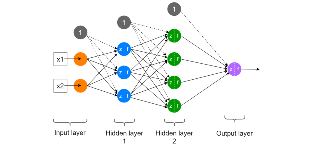
An MLP is composed of an input layer, one or more hidden layers, and an output layer. Each layer is made up of one or more perceptrons, and each perceptron in a given layer is connected to all the perceptrons in the previous layer. The hidden layers are responsible for transforming the input data into a more useful representation, while the output layer produces the final output.

MLPs are powerful models that can learn complex relationships between inputs and outputs. They have been used for a wide range of applications, such as image recognition, natural language processing, and financial forecasting. However, they can be prone to overfitting, especially if the number of hidden layers and neurons is not properly tuned, and they may require a large amount of training data to achieve good performance.

MLP Deep Learning Classification Model

Here’s an example code for classifying some data points using TensorFlow and a Multilayer Perceptron (MLP) model. First, we generate 10 random data points for (x, y), and assigns them to two classes, and plots the data points:

import numpy as np
import matplotlib.pyplot as plt

# Define the number of data points
num_points = 10

# Define the boundaries of the two classes
class1_x_min, class1_x_max = 0, 5
class1_y_min, class1_y_max = 0, 5
class2_x_min, class2_x_max = -5, 0
class2_y_min, class2_y_max = -5, 0

# Generate the data points
x1 = np.random.uniform(class1_x_min, class1_x_max, num_points // 2)
y1 = np.random.uniform(class1_y_min, class1_y_max, num_points // 2)
x2 = np.random.uniform(class2_x_min, class2_x_max, num_points // 2)
y2 = np.random.uniform(class2_y_min, class2_y_max, num_points // 2)
x = np.concatenate((x1, x2))
y = np.concatenate((y1, y2))
labels = np.concatenate((np.zeros(num_points // 2), np.ones(num_points // 2)))

# Shuffle the data points
indices = np.arange(num_points)
np.random.shuffle(indices)
x = x[indices]
y = y[indices]
labels = labels[indices]

# Plot the data points
plt.scatter(x, y, c=labels, cmap='viridis')
plt.xlabel('x')
plt.ylabel('y')
plt.show()

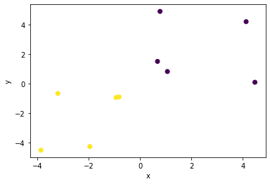
This code generates a set of 10 random data points for (x, y) that belong to two classes, and plots the data points. Note that the exact locations of the data points and the boundaries of the two classes are randomly generated and will be different each time you run the code.

import tensorflow as tf

# Define the data
# Concatenate the x and y arrays into a single (x, y) array
x_train = np.column_stack((x, y))

y_train = np.array(labels)

# Define the MLP model
model = tf.keras.models.Sequential([
  tf.keras.layers.Dense(2, activation=tf.nn.relu),
  tf.keras.layers.Dense(1, activation=tf.nn.sigmoid)
])

# Compile the model
model.compile(optimizer='adam', loss='binary_crossentropy', metrics=['accuracy'])

# Train the model
history = model.fit(x_train, y_train, epochs=1000, verbose=0)

Let me explain the code in more detail:

• We define the training data x_train and y_train. In this example, we have ten data points, where each data point is a two-dimensional vector and each target is a binary label.
• We define the MLP model using the Sequential class of TensorFlow. This model has two hidden layers with ReLU activation and a single output layer with sigmoid activation. Note that the input shape of the model is determined automatically from the input data.
• We compile the model using the binary cross-entropy loss function and the Adam optimizer. We also specify the accuracy as a metric to monitor during training.
• Next, we train the model using the fit method of TensorFlow. We use 1000 epochs for training.

Finally, we calculate the accuracy of the model using the evaluate method of Keras. This method returns the loss and the accuracy of the model on the training data, and we print the accuracy to the console.

# Calculate the accuracy of the model
loss, accuracy = model.evaluate(x_train, y_train)
print('Accuracy:', accuracy)

We can plot the model’s loss and accuracy during training using the plot function of Matplotlib. We get the values of the loss and accuracy from the history object that is returned by the fit method, and we add axis labels and a legend to the plot using the xlabel and legend functions.

# Plot the model loss and accuracy
plt.plot(history.history['loss'], label='loss')
plt.plot(history.history['accuracy'], label='accuracy')
plt.xlabel('Epoch')
plt.legend()
plt.show()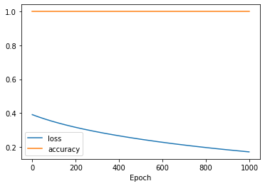

We can predict the class of new data points using this code:

# Predict some data
x_test = np.array([[-2, -2], [-3, -1], [2, 2], [2, 4]])
y_pred = model.predict(x_test)

print(y_pred)

Model architecture Visualization

To visualize the model architecture, you can use the plot_model function from the tensorflow.keras.utils module. Here’s an example code that shows how to use this function:

from keras.utils import plot_model

# Plot the model architecture
plot_model(model, show_shapes=True, show_layer_names=True)

Let me explain the code in more detail:

• We import the necessary libraries: TensorFlow and plot_model function from tensorflow.keras.utils module.
• We define the MLP model using the Sequential class of TensorFlow. This model has two hidden layers with ReLU activation and a single output layer with sigmoid activation. Note that the input shape of the model is determined automatically from the input data.
• Finally, we use the plot_model function to visualize the model architecture. The show_shapes argument is set to True to display the shapes of the input and output tensors of each layer, and the show_layer_names argument is set to True to display the name of each layer.

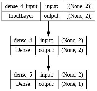
This will generate a graphical representation of the model architecture, which can be saved to a file or displayed on the screen. The output will be a visualization of the model architecture as a directed acyclic graph, with the input layer at the leftmost side, the output layer at the rightmost side, and the hidden layers in between. The arrows between the layers represent the flow of data through the network.

Tips on building MLP Model

Building a Multi-Layer Perceptron (MLP) involves several steps that can impact the performance and accuracy of the model. Here are some tips to keep in mind when building an MLP:

1. Define the problem: Clearly define the problem you are trying to solve, and determine the appropriate input and output data format.
2. Choose the right activation functions: Activation functions play a critical role in MLPs. They help to introduce non-linearity into the model and determine the output of each neuron. Common activation functions include sigmoid, ReLU, and tanh. Choose the right activation function based on the problem and data you are working with.
3. Choose the right loss function: The loss function is used to measure the difference between the predicted output and the actual output. Common loss functions include mean squared error, cross-entropy, and binary cross-entropy. Choose the right loss function based on the type of problem you are working with.
4. Choose the right optimizer: The optimizer is used to update the weights in the MLP during training. Common optimization algorithms include stochastic gradient descent (SGD), Adam, and RMSprop. Choose the right optimizer based on the problem and data you are working with.
5. Choose the right number of layers and neurons: The number of layers and neurons in an MLP can have a significant impact on its performance. A good rule of thumb is to start with a few layers and neurons and gradually increase them until you start to see diminishing returns in performance.
6. Use dropout regularization: Dropout regularization is a technique that can help to prevent overfitting in MLPs. It works by randomly dropping out a percentage of neurons during training, forcing the remaining neurons to learn more robust features.
7. Monitor the training process: Monitor the training process by tracking the loss and accuracy of the model on the training and validation sets. This will help you to identify potential problems and make adjustments to the model as needed.
8. Evaluate the model: Evaluate the performance of the model on a separate test set to determine its accuracy and generalization ability. Use a range of evaluation metrics, including precision, recall, F1 score, and accuracy, to get a comprehensive view of the model’s performance.

By following these tips, you can build an MLP that is accurate, efficient, and robust. Keep in mind that building a good MLP requires a balance of art and science, so be prepared to experiment and iterate until you find the best approach for your specific problem and data.